Credit Risk Using the Merton Model

Introduction

The Merton model is one of the most popular structural models of default. It models the equity of a firm as a European call option on its asset with the value of liabilities as the strike price. We use the option pricing mechanism in which firms asset is the underlying for the option. Under the Merton model the firm defaults when the market value of its assets fall below a given level (total liability).

The model assumes that the asset value, $A_t$, follows a Geometric Brownian motion (GBM)

\[dA_t=\mu A_tdt + \sigma A_t dW_t,\]

where $\mu$ is the mean rate of return in the asset and $\sigma$ is its volatility and $(W_t)_{t>0}$ is a Brownian motion.

After a little bit of calculus we can get

\[A_T = A_0\exp\left\{\left(\mu-\frac{1}{2}\sigma^2\right)T+\sigma W_T\right\},\]

which is the evolution of the asset value.

Many large and mid-cap firms are financed by equity and debt. Assume that the firm’s financed by one outstanding debt obligation of face value $K$ with maturity $T$ and one equity $E$. The value of the the firm is therefore given by

\[A_0 = E_0 + K_0.\]

Here $(E_t)_{t \geq 0}$ also follows a GMB, describing the evolution of the equity. $(K_t)_{t\geq 0}$ is a stochastic process describing the market value of the firm’s debt obligation.

We assess the riskiness of the firm from the debt holders’ point of view. Credit risk arises when the

\[P(A_T<F)>0.\]

This means that at maturity, $T$, the value of firm’s assets is not sufficient enough to cover the debt payment of $F$ with a positive probability. That is, the default probability is greater than zero.

We now have two cases:

1. $A_T > F$: The debt holders get the face value of $F$, the equity holders get the difference, $E_T=A_T-F$ which means there is no default.
2. $A_T \leq K$: The firm cannot meet its debt obligation. At this point, equity holders lose out, that is, $E_T=0$ and the bond holders get $F=A_T$.

---

Equity Value and Probability of Default

From the two cases above, the payoff to the shareholders at maturity $T$ is given by

\[E_T = \max\{A_T - K, 0\}.\]

The equation can be viewed as a European call option on the firm’s asset with strike price $K$ equal to the face value of the debt obligation.

The debt holders, on the other hand, receive $\min\{A_T,K\}$. We can now use the Black-Scholes formula to find the current equity (call) price

\[E_0 = A_0N(d_1)-Ke^{-rT}N(d_2),\]

where

\[d_1 = \frac{\ln\left(\frac{A_0}{K}\right)+\left(r+1/2\sigma^2\right)T}{\sigma \sqrt{T}},\]

and

\[d_2 = d_1 - \sigma\sqrt{T}.\]

One nice property of the Black-Scholes model is that the risk-neutral probability of a exercising a call option at $T$ is $N(d_2)$. Hence, the probability of not exercising the call option is $N(-d_2)$, which means that the value of debt liability $K$ is greater than the value of assets $A$. This is a firms default as mentioned earlier. In the Merton model, the probability of default is

\[\begin{aligned} PD &= P(A_T\leq K)\\ &=N\left[\frac{\ln\left(\frac{K}{E_0}\right)-\left(r-\frac{1}{2}\sigma^2 \right)T}{\sigma^2\sqrt{T}}\right] \\ &= N(-d_2). \end{aligned}\]

See more at Merton Model (1974).

Implementation in R

Simulating GBM Paths

I simulate sample paths of an equity which follows a GBM. To make my life easier, I use the R package sde to simulate the stochastic differential equation.

library(sde)
library(ggplot2)
library(ggthemes)

# GBM Parameters
N = 364  # Number of days in a year minus day 1
Tm <- 1  
A0 <- 100
mu <- 0.03

sigma <- 0.20  # volatility
r <- 0.05  # risk-free interest rate
K <- 85  # Strike price


nsims <- 100
pathMatrix <- matrix(NA, nrow = N + 1, ncol = nsims)

# GBM function in the sde package simulates a single Geometric Brownian motion path

for (i in 1:nsims) {
  pathMatrix[, i] <- GBM(x = A0, r = r, sigma = sigma, T = Tm, N = N)
}

autoplot(zoo(pathMatrix), facets = NULL) +
  theme_fivethirtyeight() +
  labs(title = "Simulated asset price paths") +
  theme(
    legend.position = "none",
    axis.line.x = element_line(linetype = "dashed"),
    panel.grid.minor.y = element_line(colour = "grey70", linetype = "dotted")
  )

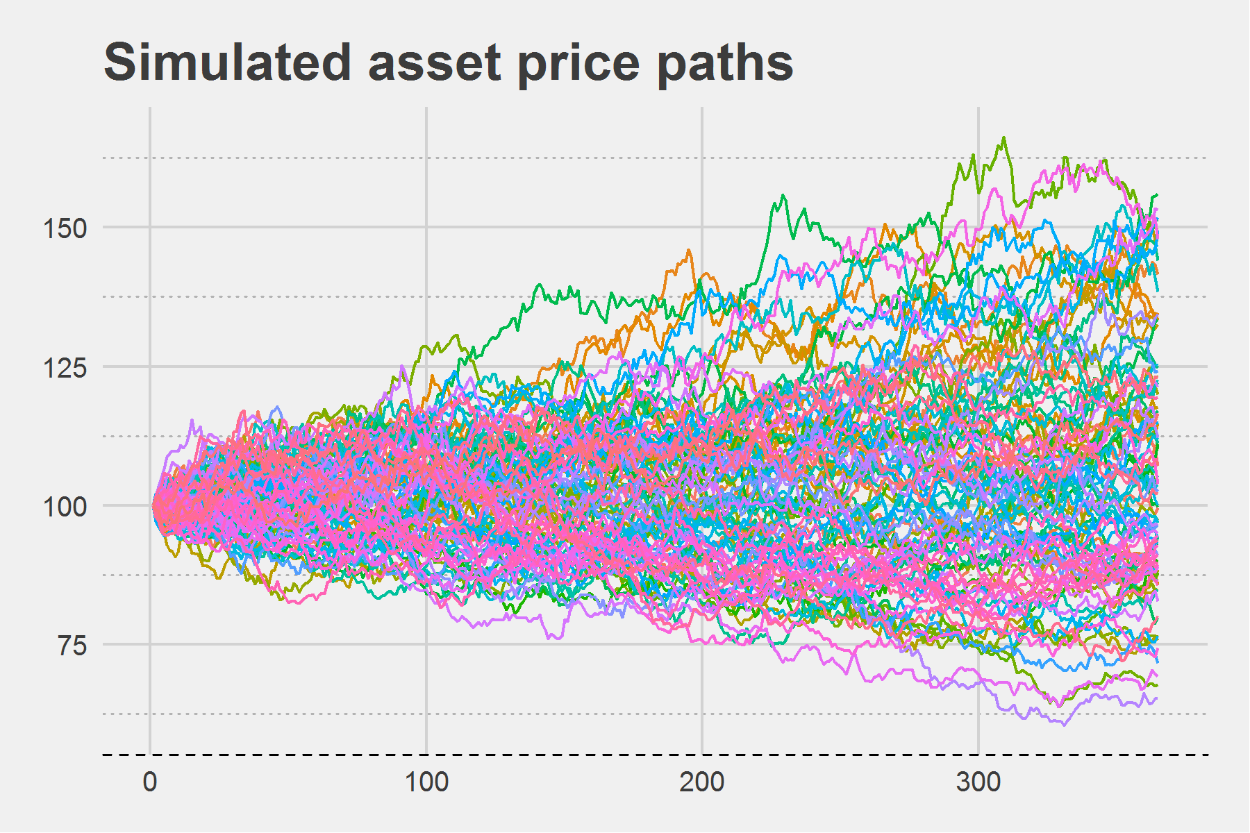
I model a distribution of the value of the asset at maturity $T$ by simulating a number of paths.

# Asset value at maturity
asst.Mty <- pathMatrix[nrow(pathMatrix), ]  # collect the asset values from each path

ggplot(data = as.data.frame(asst.Mty), aes(asst.Mty)) +
  geom_density(colour = "#276c8e", size = 0.8) +
  theme_fivethirtyeight() +
  scale_x_continuous(limits = c(50, 200)) +
  labs(title = "Probability Density of Asset value at Maturity",
       x = "Asset Value") +
  theme(
    axis.title = element_text()
  )
  

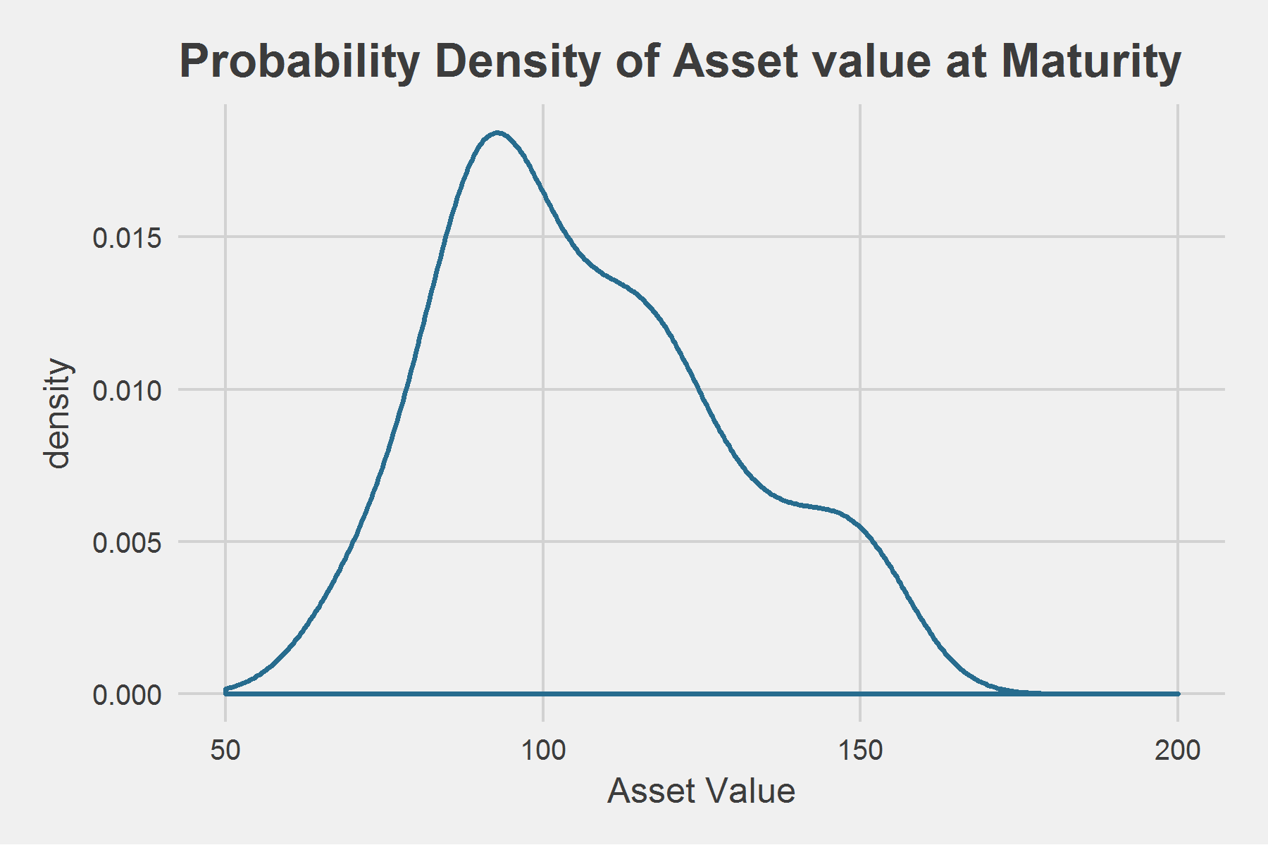
The area to the left of the vertical line, $K=85$, is the probability of default. Default occurs when the asset value at maturity falls below 85. Under the Merton model that probability is precisely $N(-d_2)$ which I compute below.

First, I write a function BSM to price the call option using the Black-Scholes model.

BSM <- function(t, A0, K, r, sigma){
  # Computes the price of a call option using Black-Schole model and
  # Probability of default for the Merton Model.
  # 
  # Args: 
  #   t:      Time in years.
  #   A0:     Asset price at time = 0.
  #   K:      Strike price (total value of debt).
  #   r:      Risk-free interest rate.
  #   sigma:  Volatility of asset value.
  #
  # Returns:
  #   Call option price.
  d1 <-  (log(A0 / K) + (r + sigma^2 / 2) * t) / (sigma * sqrt(t))
  d2 <-  d1 - sigma * sqrt(t)
  ET <- A0 * pnorm(d1) - K * exp(-r * t) * pnorm(d2)
  cbind(
    call.price = ET,
    prob.default = pnorm(-d2)
  )
}

BSM(t = 1, A0 = 100, K = 85, r = 0.05, sigma = 0.20)

Additional Information: Computing the Greeks:

There are quantities that describe derivative risk sensitivities. They represent the sensitivity value of an option to changes in underlying parameters. I won’t go into detail explaining what each one of them means. Consult Stochastic Calculus for Finance II by Shreve.

BSMGreeks <- function(t, A0, K, r, sigma){
  d1 <-  (log(A0 / K) + (r + sigma^2 / 2) * t) / (sigma * sqrt(t))
  d2 <-  d1 - sigma * sqrt(t)
  
  cbind(
    delta =  pnorm(d1),
    theta =  (-r * K * exp(-r * t * pnorm(d2))) - sigma * A0 * dnorm(d1) / (2 * sqrt(t)),
    gamma =  dnorm(d1) / (sigma * A0 * sqrt(t)),
    vega  =  A0 * sqrt(t) * dnorm(d1),
    rho   =  t * K * exp(-r * t) * pnorm(d2)
    )
}

print(BSMGreeks(t = 1, A0 = 100, K = 85, r = 0.05, sigma = 0.20), digits = 3)

Note:

• This was just an outline of of the Merton’s corporate credit risk model. I have not discussed the shortcomings of the model. There are a number of extensions to this model which is a subject for another blog post.
• Other concepts associated with this model include distance-to-default, interest rate process, expected default frequency (EDF) and sensitivity analysis.